Model-Based RL — Experiments on the Limits of Dyna-Q

This experiment does not pass planning compute off as environment samples. The central question: under a fixed real-interaction budget, how do model quality and planning allocation jointly determine the gains? It validates the core claims of model-based-rl.tex:

1. Sample efficiency: greedy-evaluated returns for different planning budgets \(n\) under a fixed number of real steps (CliffWalking, deterministic transitions);

2. Data vs compute: the benefit of planning and its wall-clock cost;

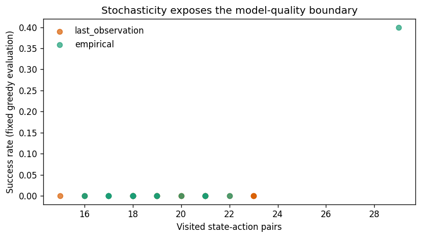
3. Model bias: on a stochastic environment (FrozenLake), the difference between last-observation and empirical count models.

All training curves are aligned by real environment steps and evaluated at fixed checkpoints with exploration-free greedy policies.

Output figures:

• fig1_sample_efficiency.pdf

• fig2_planning_sweep.pdf

• fig3_model_bias.pdf

from pathlib import Path
import json
import tempfile
import time
import numpy as np
import matplotlib.pyplot as plt
import gymnasium as gym

OUTDIR = Path('.')
RAW_RESULTS = Path(tempfile.gettempdir()) / 'breakrl-model-based-rl' / 'dyna_q_raw_results.json'
SEEDS = list(range(42, 62))
PLANNING_STEPS = [0, 1, 5, 20, 50]
CHECKPOINTS = np.arange(0, 2001, 100)
GAMMA, ALPHA, EPSILON = 0.95, 0.1, 0.1
EVAL_EPISODES = 20
plt.rcParams.update({'font.family': 'DejaVu Sans', 'figure.dpi': 120})

def q_update(q, s, a, r, ns, terminated):
    target = r if terminated else r + GAMMA * np.max(q[ns])
    q[s, a] += ALPHA * (target - q[s, a])


def evaluate(env, q, seed, episodes=EVAL_EPISODES):
    values, lengths = [], []
    for i in range(episodes):
        state, _ = env.reset(seed=seed * 1000 + i)
        total = 0.0
        for length in range(1, 201):
            state, reward, terminated, truncated, _ = env.step(int(np.argmax(q[state])))
            total += reward
            if terminated or truncated:
                break
        values.append(total); lengths.append(length)
    return float(np.mean(values)), float(np.mean(lengths)), float(np.mean(np.asarray(values) > 0))


def train_dyna(env_name, planning_steps, seed, model_kind='empirical', total_steps=2000):
    train_env = gym.make(env_name, is_slippery=(env_name == 'FrozenLake-v1'))
    eval_env = gym.make(env_name, is_slippery=(env_name == 'FrozenLake-v1'))
    if hasattr(train_env.action_space, 'seed'):
        train_env.action_space.seed(seed)
    if hasattr(eval_env.action_space, 'seed'):
        eval_env.action_space.seed(seed + 100000)
    rng = np.random.default_rng(seed)
    q = np.zeros((train_env.observation_space.n, train_env.action_space.n))
    model, seen = {}, []
    records = []
    state, _ = train_env.reset(seed=seed)
    started = time.perf_counter()
    for step in range(total_steps + 1):
        if step in CHECKPOINTS:
            score, length, success = evaluate(eval_env, q, seed, episodes=EVAL_EPISODES)
            records.append({'step': step, 'eval_return': score, 'eval_length': length, 'success': success,
                            'planning_updates': step * planning_steps, 'coverage': len(seen),
                            'wall_seconds': time.perf_counter() - started})
        if step == total_steps:
            break
        action = int(rng.integers(train_env.action_space.n)) if rng.random() < EPSILON else int(np.argmax(q[state]))
        ns, reward, terminated, truncated, _ = train_env.step(action)
        episode_done = terminated or truncated
        q_update(q, state, action, reward, ns, terminated)
        key = (int(state), action)
        if key not in model:
            seen.append(key)
            model[key] = []
        model[key].append((int(ns), float(reward), bool(terminated)))
        for _ in range(planning_steps):
            ps, pa = seen[rng.integers(len(seen))]
            outcomes = model[(ps, pa)]
            if model_kind == 'last_observation':
                pns, pr, p_terminated = outcomes[-1]
            else:
                pns, pr, p_terminated = outcomes[rng.integers(len(outcomes))]
            q_update(q, ps, pa, pr, pns, p_terminated)
        state, _ = train_env.reset(seed=seed + step + 1) if episode_done else (ns, {})
    train_env.close()
    eval_env.close()
    return records, q, model


def run_condition(env_name, n, model_kind='empirical'):
    rows = []
    for seed in SEEDS:
        records, _, model = train_dyna(env_name, n, seed, model_kind=model_kind)
        for row in records:
            rows.append({'seed': seed, 'n': n, 'model': model_kind, **row})
    return rows

---

Figure 1 — Sample efficiency: the benefit of planning under fixed real steps

Evaluation curves for different planning budgets \(n\) on CliffWalking-v0 (greedy evaluation over 20 seeds; the x-axis is real environment steps, not episode numbers): in a deterministic environment the model is exactly right — the more planning steps, the farther the same real data propagates and the faster the convergence.

# Experiment 1: fixed real-step evaluation on deterministic CliffWalking.
rows = [row for n in PLANNING_STEPS for row in run_condition('CliffWalking-v0', n)]
means = {}
for n in PLANNING_STEPS:
    subset = [r for r in rows if r['n'] == n]
    means[n] = (np.array([r['eval_return'] for r in subset]).reshape(len(SEEDS), -1).mean(axis=0),
                np.array([r['eval_return'] for r in subset]).reshape(len(SEEDS), -1).std(axis=0))
fig, ax = plt.subplots(figsize=(7, 4))
for n, (mean, std) in means.items():
    ax.plot(CHECKPOINTS, mean, label=f'n={n}')
    ax.fill_between(CHECKPOINTS, mean - std, mean + std, alpha=.12)
ax.set(xlabel='Real environment steps', ylabel='Greedy evaluation return', title='Planning helps only when the learned model is useful')
ax.legend(ncol=3, frameon=False)
fig.tight_layout(); fig.savefig(OUTDIR / 'fig1_sample_efficiency.pdf', bbox_inches='tight'); plt.show()

---

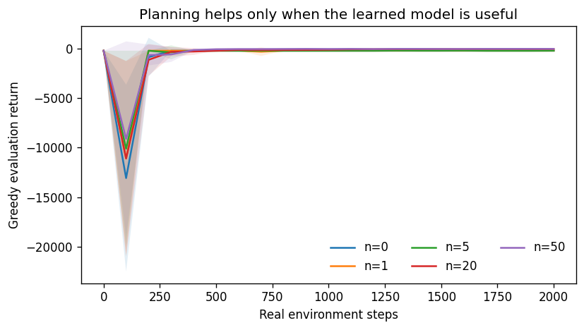
Figure 2 — Data and compute: the benefit and cost of planning steps

Final greedy return (left) and wall-clock time (right) after the same 2000 real environment steps (20 seeds per \(n\)): planning’s benefit grows with \(n\) but with diminishing returns, while the compute cost grows nearly linearly — simulated updates are not new samples; the benefit is essentially “squeezing the data dry”.

# Experiment 2: data versus computation. Report both real steps and planning updates.
final_rows = [r for r in rows if r['step'] == CHECKPOINTS[-1]]
fig, axes = plt.subplots(1, 2, figsize=(10, 4))
for n in PLANNING_STEPS:
    subset = [r for r in final_rows if r['n'] == n]
    scores = np.array([r['eval_return'] for r in subset])
    axes[0].errorbar(n, scores.mean(), yerr=scores.std(), fmt='o', capsize=4)
    axes[1].errorbar(n, np.mean([r['wall_seconds'] for r in subset]), yerr=np.std([r['wall_seconds'] for r in subset]), fmt='o', capsize=4)
axes[0].set(xlabel='Planning updates per real step (n)', ylabel='Final greedy return')
axes[1].set(xlabel='Planning updates per real step (n)', ylabel='Wall-clock seconds')
fig.suptitle('More planning trades computation for data; it does not create information')
fig.tight_layout(); fig.savefig(OUTDIR / 'fig2_planning_sweep.pdf', bbox_inches='tight'); plt.show()

---

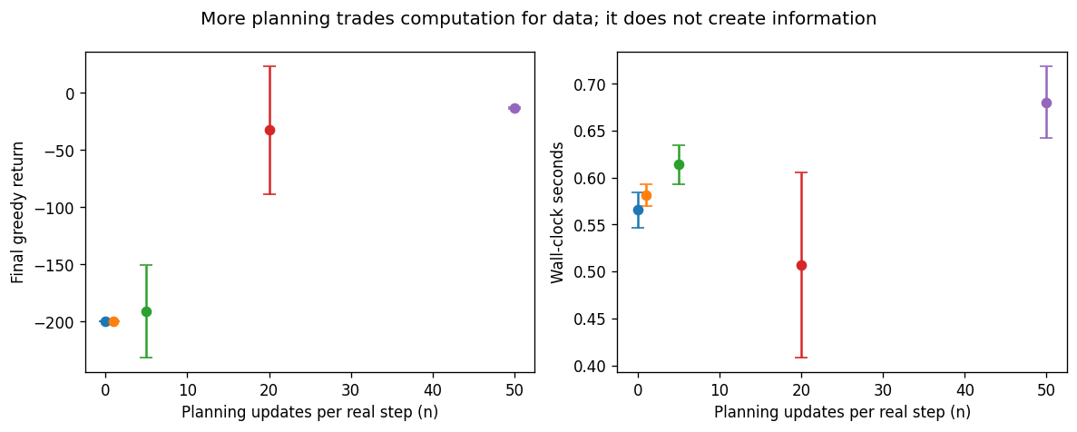
Figure 3 — Model bias: last-observation vs empirical count models

Coverage–success diagnostics on stochastic FrozenLake-v1 (each point is one seed; success rates come from a fixed, exploration-free greedy evaluation): the last-observation model records stochastic transitions as whatever was last observed, so planning overgeneralizes; the empirical count model keeps the transition uncertainty and no longer mistakes accidents for certainties. Note that (s,a) coverage is very low in this experiment — both models’ success rates are near 0; read the scatter’s shape (how model bias suppresses success), not the absolute values.

# Experiment 3: last observation versus empirical model on stochastic FrozenLake.
model_rows = []
for kind in ['last_observation', 'empirical']:
    model_rows.extend(run_condition('FrozenLake-v1', 20, model_kind=kind))
final = [r for r in model_rows if r['step'] == CHECKPOINTS[-1]]
fig, ax = plt.subplots(figsize=(7, 4))
for kind, color in [('last_observation', '#d95f02'), ('empirical', '#1b9e77')]:
    subset = [r for r in final if r['model'] == kind]
    x = np.array([r['coverage'] for r in subset]); y = np.array([r['success'] for r in subset])
    ax.scatter(x, y, alpha=.7, label=kind, color=color)
    print(kind, {'success_mean': float(y.mean()), 'coverage_mean': float(x.mean())})
ax.set(xlabel='Visited state-action pairs', ylabel='Success rate (fixed greedy evaluation)', title='Stochasticity exposes the model-quality boundary')
ax.legend(frameon=False); fig.tight_layout(); fig.savefig(OUTDIR / 'fig3_model_bias.pdf', bbox_inches='tight'); plt.show()
RAW_RESULTS.parent.mkdir(parents=True, exist_ok=True)
with RAW_RESULTS.open('w', encoding='utf-8') as handle:
    json.dump(rows + model_rows, handle, ensure_ascii=False, indent=2)

last_observation {'success_mean': 0.0, 'coverage_mean': 19.45}
empirical {'success_mean': 0.02, 'coverage_mean': 19.05}

Summary

• Planning’s benefit comes from repeatedly propagating existing experience through the model — nearly free in deterministic environments;

• The cost is compute: planning steps bring nearly linear wall-clock cost with diminishing returns;

• The premise is model quality: in stochastic environments a wrong model representation (last-observation) lets planning amplify bias — the limits of model-based methods are set by “how accurate is the model”.